
Using the Program
Table of Contents
What IntegraTax does
Congratulations! You have accumulated your DNA sequences and are ready to analyse them! You can use the test files archive to download files to figure the software out.
- Singapore_mycetophilidae_dataset1.fasta : Project fasta file from Amorim et al. 2025/Meier et al. 2025
- Singapore_mycetophilidae_dataset1.spart : Spart file generated via SpartExplorer
- BLAST_reference_myceto_genbank : Uncurated references from GenBank for Mycetophilidae.
IntegraTax has two modules:
1. Clustering: Groups your sequences into sets of speciemen based on pairwise distances hierarchically (single linkage/ Objective clustering)
2. Taxonomy: For annotation of the clusters and specimens as a dendrogram (Cluster Fusion Diagram).
First lets take the sequences through module 1 which gives you several options:
Module 1: Objective clustering
Typically IntegraTax Clustering module is run in Mode 1 (one file) or Mode 2 (two input FASTA files). Additionally an experimental Mode 3 is implemented to help you clean up a fasta file with non overlapping regions.
Input files needed
1. FASTA file(s)
- There no length limit to sequence headers but it would be beneficial to keep them organized. If you have specimen codes, the format compatible with IntegraTax is alphanumeric, such as ZRC00001 or similar to accession codes in GenBank. FASTA file can be aligned or not unaligned.
NOTE: If you have a 2nd fasta file with identified reference sequences for Mode 2 (e.g. from NCBI genbank or BOLD or sequences from other projects), IntegraTax can add those sequences to the clustering in Step 3. This file need not be aligned as this mode is always run with pairwise alignments
2. Species name file (optional)
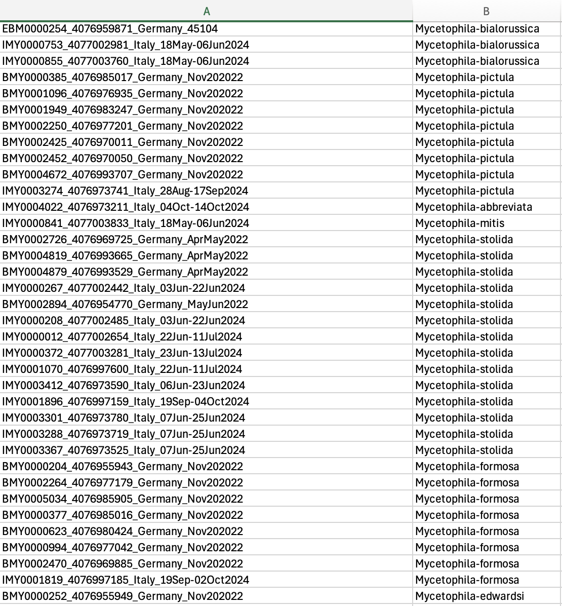
- Only required if you want manual species name detection instead of automatic extraction.
- Format: A .tsv (tab delimited) file containing species names that corresponds to your sequence headers Example: Column A is your sequence header, column B is your species name.
Clustering
1. Open IntegraTax.
Haven’t installed it yet? Go to the installation page.
2. Select the aim of your project
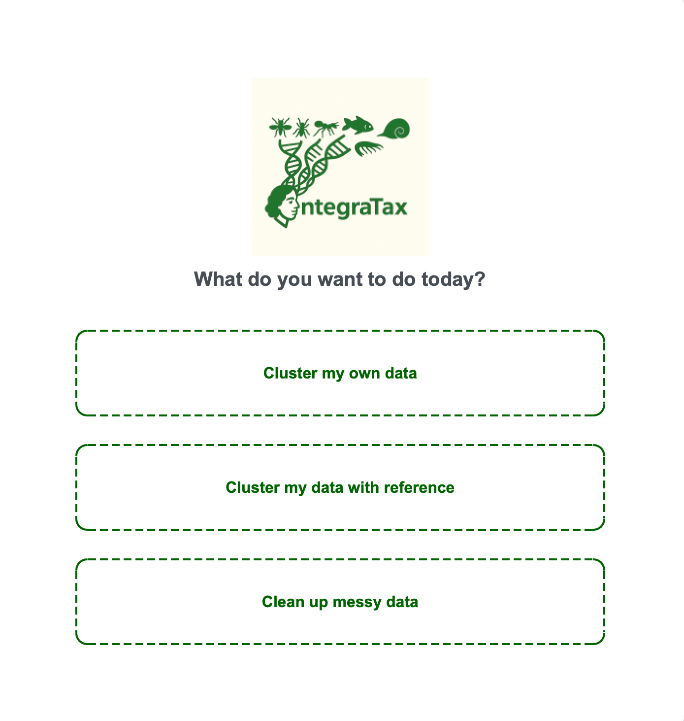
IntegraTax offers you 3 modes. Click as needed
- Mode 1: You have a set of sequences for specimens you want to study. The sequences are curated, i.e. you know they are overlapping and are of the target region
- Mode 2: You have sequences for Mode 1, but also want to include some reference sequences that came from earlier studies (e.g. NCBI/BOLD)
- Mode 3: You are in an exploratory phase, have downloaded data from GenBank and want to clean it up to overlapping regions. You can clean up the data and cluster.
Mode 1
Mode 1 Step 1. Drag your FASTA file into the box
Mode 1 Step 2. If you have sequences of equal length (incl., if present, gaps), you will see a pop-up. Otherwise, proceed to Mode 1 Step 3
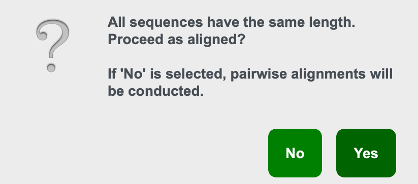
- If your sequences are already aligned, select Yes.
- Otherwise, select No.
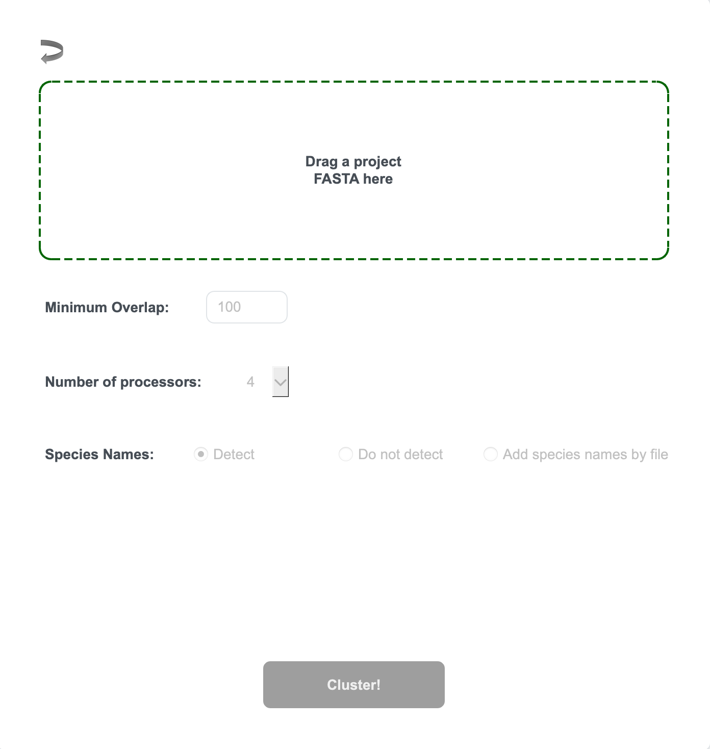
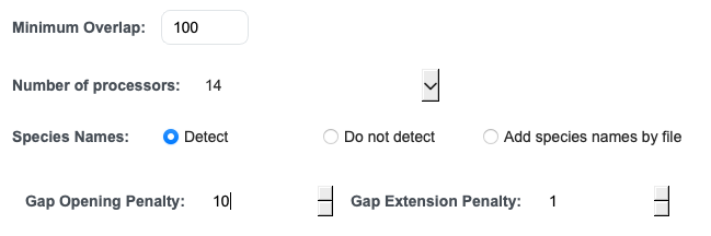
Mode 1 Step 3. Set up your clustering configuration

- Overlap length setting (Minimum Overlap)
- This is crucial because the software will alert if it finds too many short overlaps. It insists on having at least some minimum overlaps between fragments.
- Number of processors
- Number of processors used for distance calculations. This matters especially for large datasets.
- Species name detection
- Automatic (from FASTA headers): Click “Detect”
- Manual: Click “Add species name by file” and select your species name file
- No detection: Click “Do not detect”
- Gap opening and extension penalty (pairwise alignment mode only)
- Allows you to modulate alignment parameters for pairwise alignment
Mode 1 Step 4. Click “Cluster” to begin.
- After the clustering the dendrogram viewer .html will open automatically for visualisation (Module 2: Taxonomy)
- Refer to Clustering Output files for details of the outputs.
Mode 2
This mode is for when you have 2 FASTA files (project and reference files)
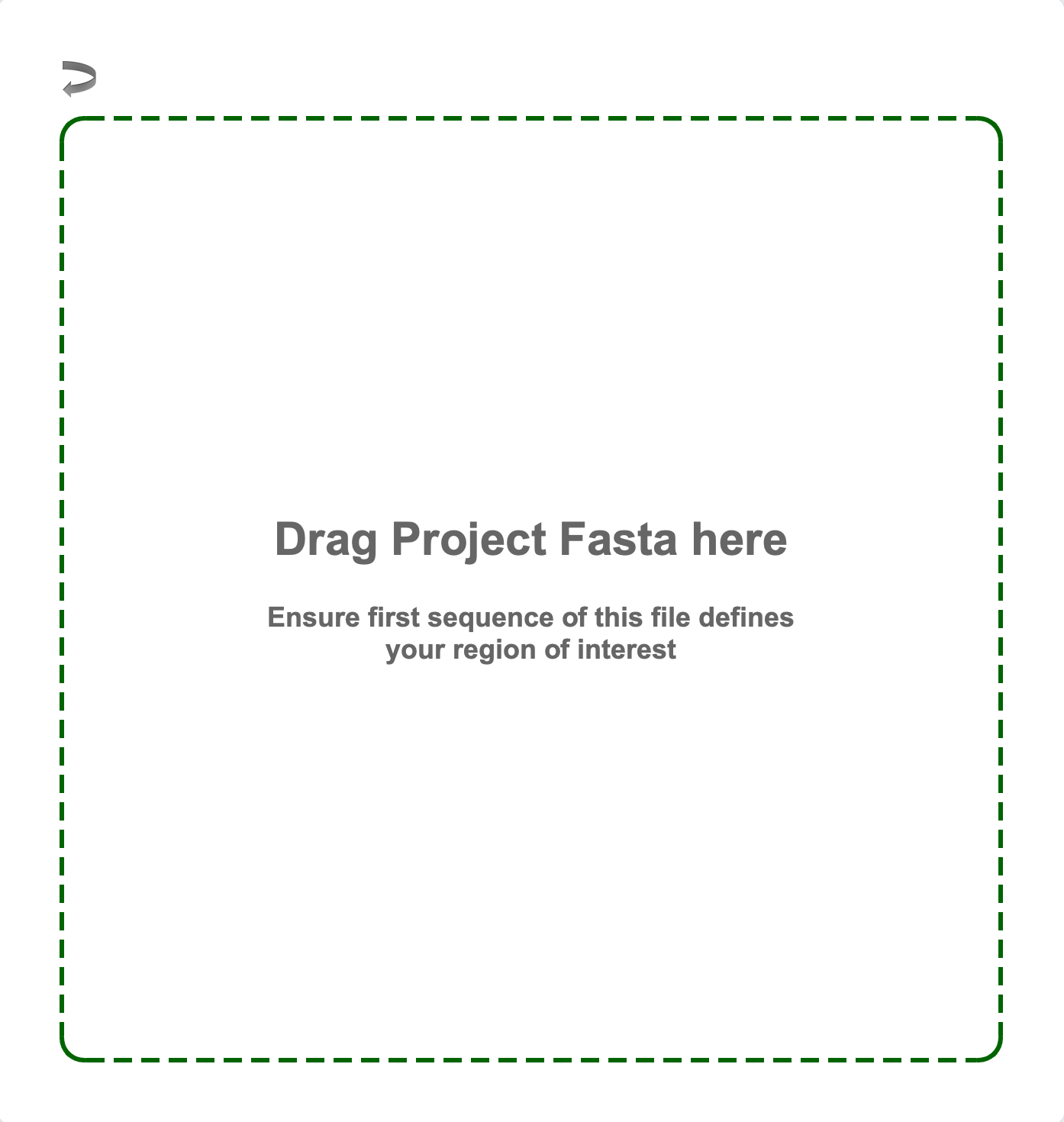
Mode 2 Step 1. Drag your Project FASTA file into the box
You will notice an alert saying the top sequence is reference sequence. This is because we need to ensure that eventually overlapping regions make it to the dendrogram. The first sequence tunes the hit length parameter in the BLAST search done later.
Mode 2 Step 2. Drag your Reference FASTA file into the box
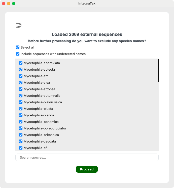
Mode 2 Step 3. Select the species you wish to include
Unselect any unwanted species and click Proceed.
Mode 2 Step 4. Select “BLAST based homology search”
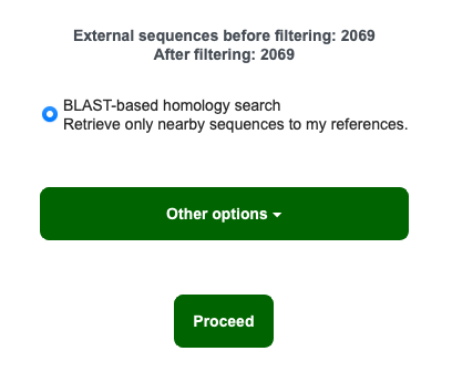
At this stage, ensure that the names of the folders where your 2nd fasta file does not have spaces. For example, in the directory /Users/Name/Desktop/GenBank Sequences/Mycetophilidae Sequences, remove the space in GenBank Sequences and Mycetophilidae Sequences or replace them with another character. If there are spaces in the directory, the BLAST based homology search will fail!
Other homology search options can be found in the “Other options” button, click HERE for more information, warnings, and instructions.
Click “Proceed” to continue.
Mode 2 Step 5. Choose your settings for BLAST based homology search
- Output prefix
- Threads
- Identity cutoff (%)
- Hit length cutoff (fraction)
- Number of hits
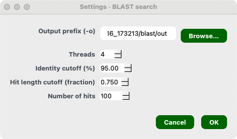
Once done, click Ok.
Mode 2 Step 6. Set the following alignment and clustering variables:
- Minimum overlap for clustering settings
- Gap opening and extension penalty for alignment settings
- Number of processors your computer can use
- Species name detection options
Mode 2 Step 7. Click “Cluster” to begin
- After the clustering the dendrogram viewer .html will open automatically for visualisation (Module 2: Taxonomy)
- Refer to Clustering Output files for details of the outputs.
Mode 3
Mode 3 is a homology search feature implemented in IntegraTax. It uses the first sequence in the input FASTA file as an initial reference and computes pairwise distances between this sequence and all other sequences (Pass 1). These distances are used to construct a distance distribution, which is smoothed using a Kernel Density Estimator (KDE). The antimode (valley) of the smoothed distribution is identified as a breakpoint, and sequences whose distances fall within overlapping regions of the distribution are trimmed.
To reduce bias introduced by relying on a single reference sequence, the procedure is repeated using N sequences (default: 10) sampled across the distance profile of the first pass (Pass 2).
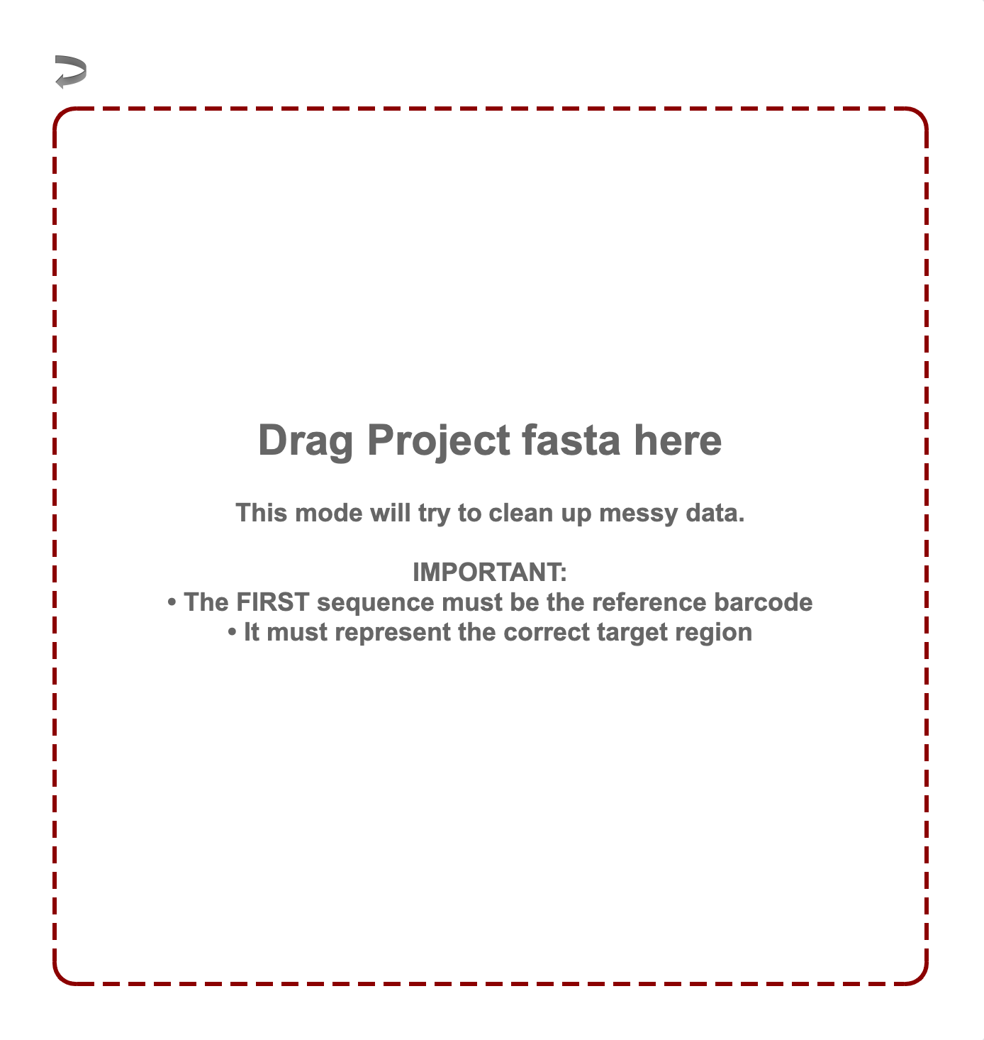
Mode 3 Step 1. Drag your FASTA file into the box
Mode 3 is going to implement a homology search feature. This will use the first sequence of your file to define the reference and trim the longer or partially overlapping region to the region of interest.
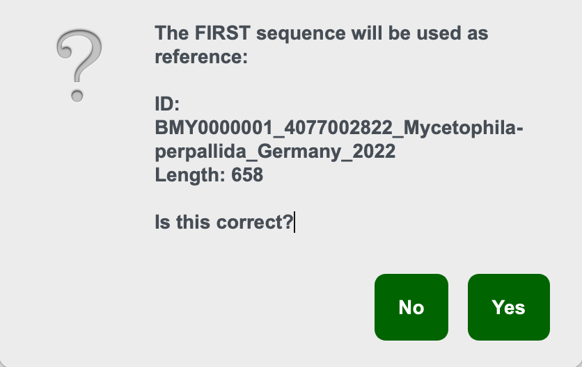
Mode 3 Step 2. On loading the first sequence ID will be printed
Confirm based on the ID
Mode 3 Step 3. Configure the search
- Output prefix: This will print the output files with this prefix
- Max proportion of N: As homology searches are based on similarity, having too many Ns in the references can influence distance calculation. You can exclude the
- Number of sequences for 2nd pass: See Mode 3 description. Number of sampled sequences.
- Min length fraction: Minimum length of overlap required to be considered a homologous fragment. 0.75 is default and this is because in fragmented landscape, this will ensure sufficient overlap between two partial sequences
- Bandwidth: The distance distribution is smoothened by a Kernel Density Estimator implemented in SciPy, where the bandwidth is selected using Silverman’s or Scott’s rule.
- KDE q_low: Lower quantile of the KDE-smoothed distance distribution used to restrict the analysis range and suppress extreme low-end outliers.
- KDE q_high: Upper quantile of the KDE-smoothed distance distribution used to restrict the analysis range and suppress extreme high-end outliers.
- Min prominence: Minimum required depth of a valley (relative to surrounding peaks) for it to be considered significant.
- Fixed threshold pass 1: By pass autodetection using fixed distance threshold (proportion)
- Fixed threshold pass 2: Same as above but for pass 2. (proportion)
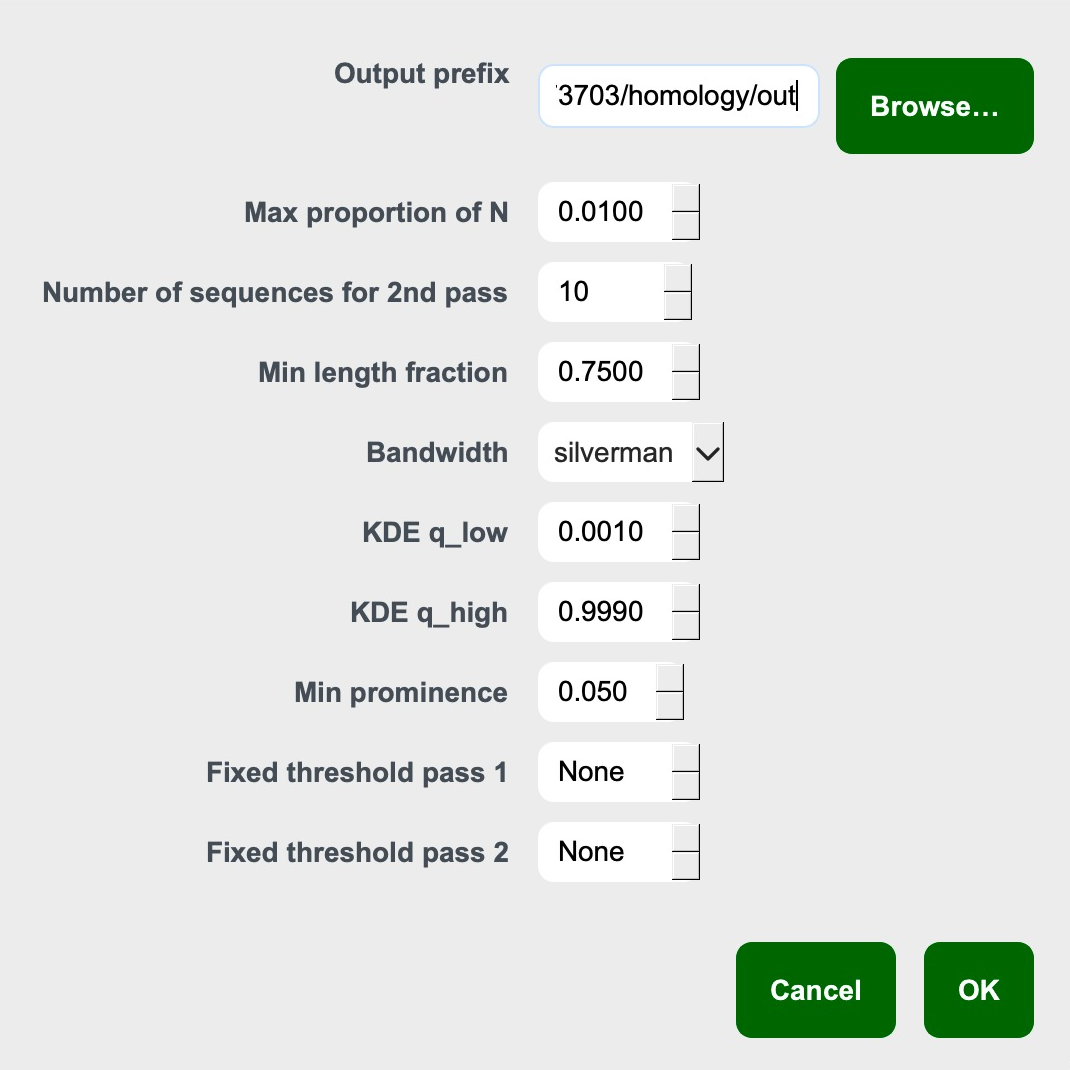
Once done, click Ok.
Mode 3 Step 4. Once homology search is done:
- Click “Save log…“ to save the log.
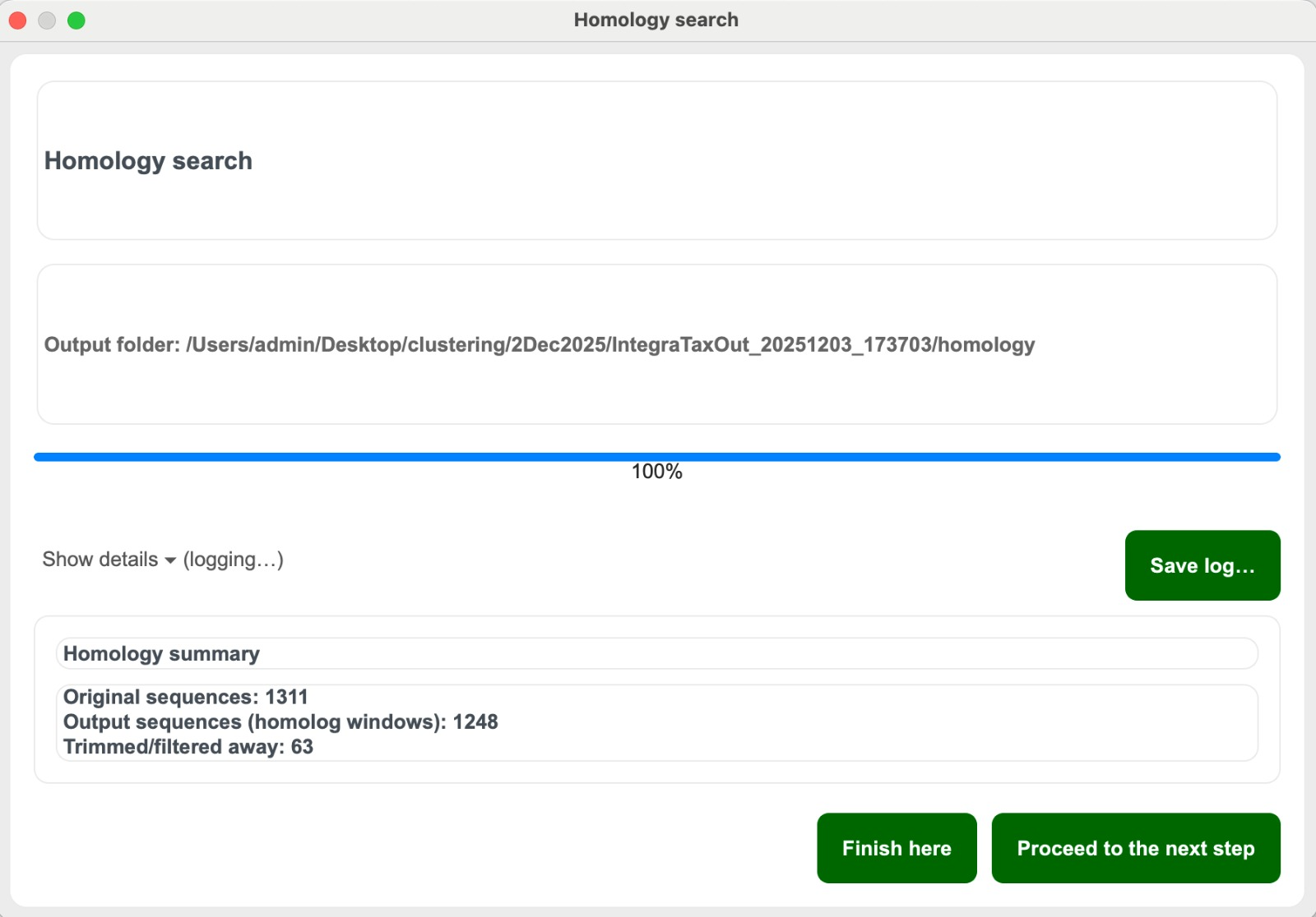
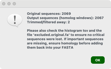
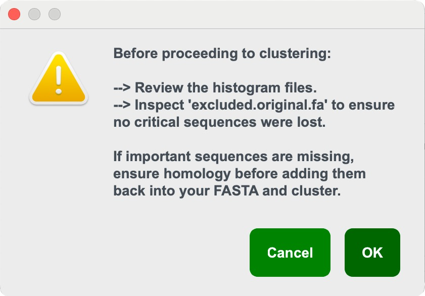
- Click “Finish here” if you want to end the process and not continue with clustering. A pop-up reminds you to review results in the “Homology” folder of the output folder. You will then be returned to the start page.
- Or click “Proceed to clustering” to move to the clustering step (Continue to Step 9).
Mode 3 Step 5. Set the following alignment and clustering variables:
- Minimum overlap for clustering settings
- Gap opening and extension penalty for alignment settings
- Number of processors your computer can use
- Species name detection options
Mode 3 Step 6. Click “Cluster” to begin
- After the clustering the dendrogram viewer .html will open automatically for visualisation (Module 2: Taxonomy)
- Refer to Clustering Output files for details of the outputs.
Other Homology Search Options with identified reference sequences
Not the right option for you? Return to Mode 2 Step 4!
-
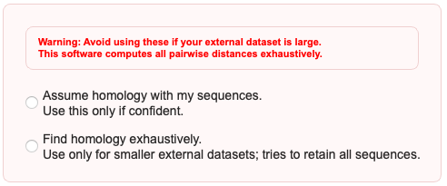
Find homology exhaustively
- If you click “Find homology exhaustively”, set the following variables:
- Output prefix: This will print the output files with this prefix
- Max proportion of N: As homology searches are based on similarity, having too many Ns in the references can influence distance calculation. You can exclude the
- Number of sequences for 2nd pass: See Mode 3 description. Number of sampled sequences.
- Min length fraction: Minimum length of overlap required to be considered a homologous fragment. 0.75 is default and this is because in fragmented landscape, this will ensure sufficient overlap between two partial sequences
- Bandwidth: The distance distribution is smoothened by a Kernel Density Estimator implemented in SciPy, where the bandwidth is selected using Silverman’s or Scott’s rule.
- KDE q_low: Lower quantile of the KDE-smoothed distance distribution used to restrict the analysis range and suppress extreme low-end outliers.
- KDE q_high: Upper quantile of the KDE-smoothed distance distribution used to restrict the analysis range and suppress extreme high-end outliers.
- Min prominence: Minimum required depth of a valley (relative to surrounding peaks) for it to be considered significant.
- Fixed threshold pass 1: By pass autodetection using fixed distance threshold (proportion)
- Fixed threshold pass 2: Same as above but for pass 2. (proportion)
Once done, click Ok.
-
Once homology search is done:
- Click “Save log…“ to save the log.
- Click “Finish here” to stop and review the “Homology” folder (you’ll return to the start page).
- Or “Proceed to clustering” (Continue to Step 8).
- Click “Save log…“ to save the log.
- If you click “Find homology exhaustively”, set the following variables:
-
Assume homology with my sequences — Go to Step 8
Use this only when you are absolutely certain that your identified reference sequences are homologous to your project sequences!!
Clustering output files
You will receive a nested folder (e.g. IntegraTaxOut_20251007_101901) in the same location as your input fasta file containing the following:
FILES
1. .itv – used for dendrogram visualisation
2. IntegraTaxViz.html – Visualisation of your dendrogram in .html format
3. external.filtered.fa (If you have identified reference sequences) – A fasta file containing your filtered identified reference sequences (after the blast homology search)
4. combined.fa (If you have identified reference sequences) – A combined fasta file containing your project sequences and your filtered identified reference sequences (after the blast homology search)
FOLDERS
1. cluster – Contains iddict.txt(mapping of IDs) and _clusterlist(Shows which sequences group into clusters across different distance thresholds)
2. pmatrix – Pairwise matrix files
3. homology (If you did a homology search without BLAST) – Contains the histogram and fasta files you should check before clustering
4. blast (If you did a homology search with BLAST) – Contains the BLAST database created from your project sequences and results of the BLAST
Module 2 Taxonomy
Once your clustering is complete, the .html dendrogram viewer opens automatically.
To begin:
- Click “Choose File” and upload the .itv file from the clustering step.
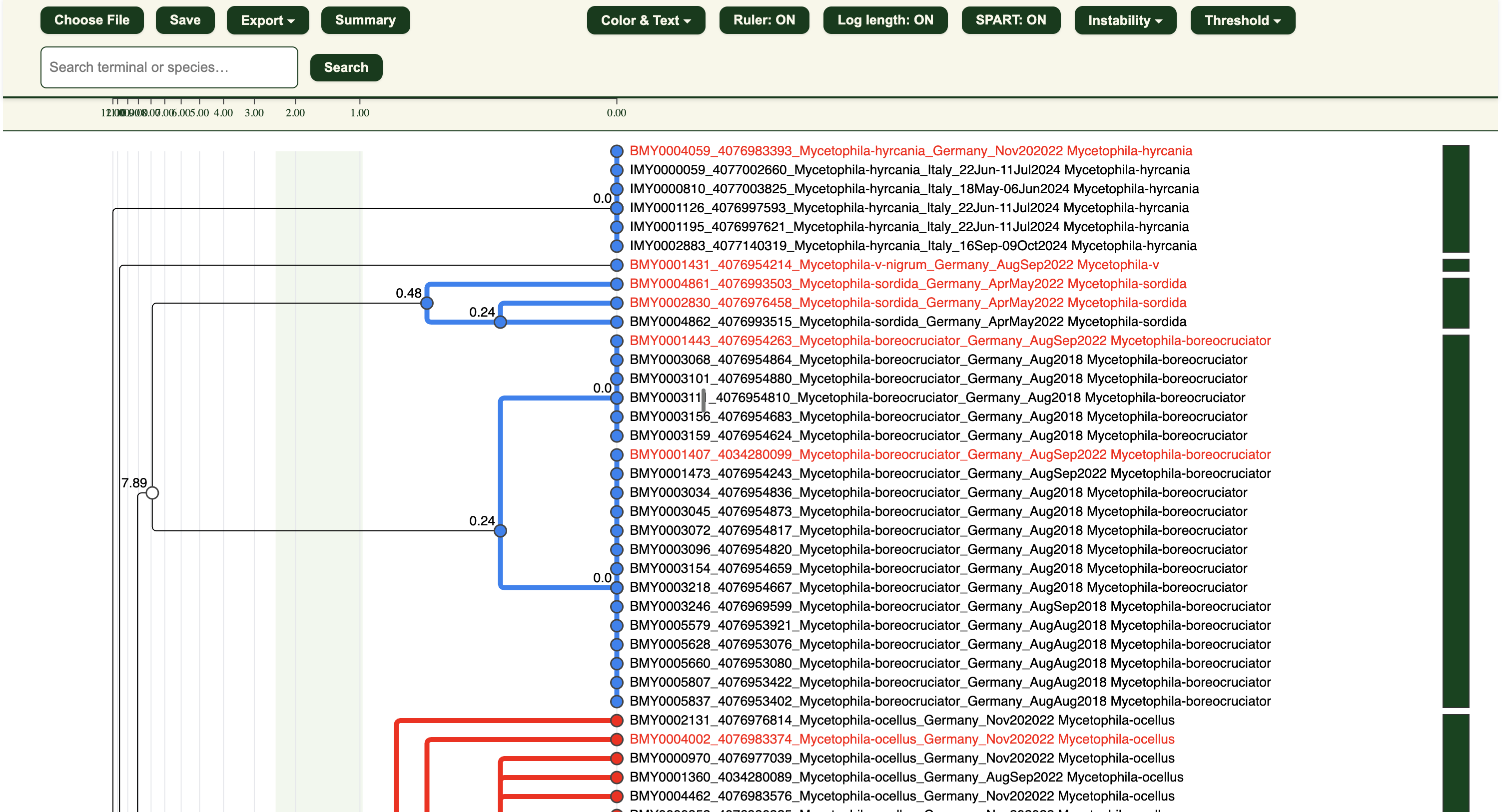
Visualisation Functions
Here are the main buttons on the top panel. Click below for more details:
- Choose File: To load the .itv for viewing
- Save: To save your visualisation as a .itv file for reloading in the future.
- Export
- Summary
- Color & Text
- Ruler: ON/OFF
- Log length: ON/OFF
- Instability
- Threshold
Export
Here are the following export formats you can choose:
-
SVG
High-resolution dendrogram image for publications or sharing. -
FASTA
Information that you have assigned such as sex, verification status, contamination etc. will be recorded in the sequence header. - Excel (LIT)
Spreadsheet with:- Cluster information
- Haplotype statistics
- Assigned species names
- Sex / holotype indicators
- LIT status
- SPART
A standardised species delimitation output format.
Summary
Here you can obtain some summary statistics for your sequences.
There will be a pop up asking if you if you would want to calculate the summary statistics for all percentage thresholds.
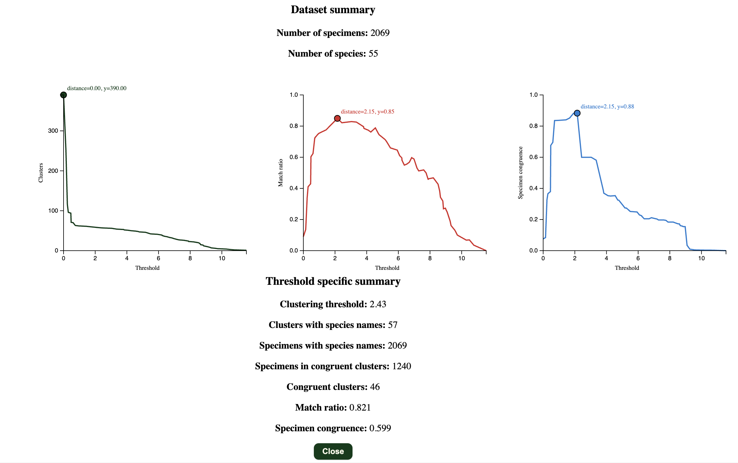
If you do not have any species names assigned to the clusters, it will only show the graph of “Clusters” against “Threshold”. If you do have species names, it will also calculate the match ratio (Species congruence) and specimen congruence.
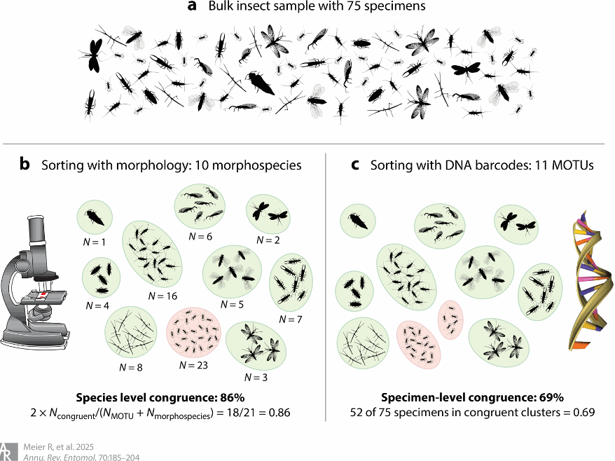
Match ratio (Ahrens et al. 2016)
where $N_{\text{congruent}}$ is the number of clusters congruent between the method and morphology, $N_{\text{morpho}}$ is the number of morphospecies, $N_{\text{method}}$ is the number of method-based clusters.
Specimen congruence (Meier et al. 2025; Derived from Yeo et al. 2020)
Color & Text
Cluster and node colours in the dendrogram are based on the LIT workflow by default.
You can edit the colours of the nodes, cluster(subtree) branches, and text here:
- Subtree colour (PI/nonPI / Binomial name / None)
- Terminal node colour (Binomial name / Cluster / Haplotype / LIT selections / None)
- Node colour (PI/nonPI / Binomial name / None):
- Text colour (Binomial name / Cluster / Haplotype / LIT selections / None)
You can change the text settings here:
- Node text: Change the numbers beside the nodes to fusepoints, MaxP(Maximum Pairwise Distance), or Node ID
- Terminal text length: Are your sequence headers too long? You can truncate it to your desired character length. Hovering your cursor over the headers will reveal the entire header.
Ruler and branch length scaling controls
Adjust the dendrogram’s scale and view thresholds for better interpretation of cluster distances.
- Ruler: ON/OFF — shows or hides pairwise distance threshold scale
- Log length: ON/OFF — toggle logarithmic branch length view
SPART visualization
You can get SPART outputs from other species delimitation approaches: For example use SPART explorer to get it for ASAP/ABGD
- Load the SPART file
- Panel: You can see the panel on the right that summarizes multiple delimtation schemes.
- It first builds a unified species delimitation where any scheme in any delimtiation gets a unique identifier.
- This is then used to show consistancy across partitions.
- The tool tip can be used to identify the cluster. Split clusters are shown with dashed boxes
Instability
Adjust your Instability maximum and minimum percentages and maximum pairwise distance (Max P) here. You can also turn the instability zone (light green background of the dendrogram) on or off. For more information about Max P and Instability, click here!
Threshold
You can adjust the clustering threshold to check the number of corresponding clusters. You can also collapse part of the dendrogram at a specific threshold of your choosing.
Right-click options
The right-click menu allows you to set verification statuses, assign metadata, and perform various actions on individual specimens or entire clusters.
Right-click on a specimen (terminal) node to:
- Set as Verified – Mark the specimen as checked and correct
- Cannot be verified – Missing or damaged specimen
- Set as Contamination – Mark as contamination if the specimen clearly belongs to a different species
- Set as Male – Indicate specimen is male
- Set as Female – Indicate specimen is female
- Set as Holotype – Mark the specimen as the holotype
- Set as Slide Mounted Specimen – Indicate the specimen is slide-mounted
- Accept code as species name – Use the specimen code as its species name
- Edit/Enter species name – Assign a user-defined species name
- Copy FASTA sequence – Copies the sequence header and sequence into clipboard
- Copy Sequence / Search online – Copies the sequence header and sequence and opens search tools for:
- Barcode of Life Data Systems (BOLD)
- NCBI (National Center for Biotechnology Information) GenBank
- Global Biodiversity Information Facility (GBIF)
- Add notes – Add any information tagged to the node
- Freeze / Unfreeze – Prevent or allow further changes to the node
- Undo – Revert the most recent change done to the node
Right-click on a cluster (internal) node to:
- Export FASTA – Download all sequences in the cluster as a .fasta file
- Accept lowest code as species name – Use the lowest specimen code of the cluster as its species name
- Enter species name – Assign a user-defined species name
- Collapse / Expand subtree – Collapse the cluster(subtree) into a single node or to show all specimens in the cluster
- Copy sequence / Search Online – Copies all headers and sequences of the cluster and opens search tools for:
- Barcode of Life Data Systems (BOLD)
- NCBI (National Center for Biotechnology Information) GenBank
- Global Biodiversity Information Facility (GBIF)
- Add notes – Add any information tagged to the node
- Freeze / Unfreeze – Prevent or allow further changes to the node
- Undo – Revert the most recent change done to the node
If the specimen (terminal) node and cluster (internal) node is shared, left-click the node to switch between both right-click options.
Saving your progress
Click the “Save” button to export a .itv save file with your edits:
- Verification status (e.g. verified, cannot be verified)
- Assigned specimen information (e.g. species names, sex, condition, type status, notes)
To resume your work, upload the .itv using the “Choose File” button.
Export formats available
-
FASTA
The labels that you set (Verification statuses, sex, holotype, contamination, slide-mounted specimens) will be noted in your sequence header. However, the notes from “Add notes” will not be in your sequence header. -
SVG
High-resolution dendrogram image for publications or sharing. Similarly, labels that you have set will be shown but notes from “add notes” will not be reflected. -
SPART
A standardised species delimitation output format. -
Excel (LIT)
Spreadsheet with 9 columns:- ID: Sequence header
- SpName: Corresponding species name that IntegraTax has detected or you have assigned
- Haplotype: The name of the haplotype cluster the particular specimen is in based on the “lowest” sequence name
- LIT selection: Specimens that IntegraTax suggests for checking based on LIT
- Cluster: Cluster number based on your chosen percentage threshold
- Sex: Male or female based on your input from the right-click options
- Holotype: Holotype or not(blank) based on your input from the right-click options
- Status: “Verified”, “Cannot be verified”, “Contamination”, “Slide Mounted” or blank based on your input from the right-click options
- Notes: Contains any notes you have added from the right-click options